Category Archives: Pandas

Binning with Pandas

This article will review two powerful and timesaving methods available from Pandas and Numpy that can be applied to problems that frequently arise in Data Analysis. These techniques are especially applicable to what is sometimes called ‘binning’ -transforming continuous variables into categorical variables.

The two methods are np.select() and pd.cut(). I call these Pandas tricks, but some of the actual implementation is taken from Numpy and applied to a Pandas container.

np.select()

Most Pandas programmers know that leveraging C-based Numpy vectorizations is typically faster than looping through containers. A vectorized approach is usually simpler and more elegant as well–though it may take some effort to not think in terms of loops. Let’s take an example of assigning qualitative severity to a list of numerical vulnerability scores using the First.org CVSS v3 mapping:

RatingCVSSv3 Score
None0.0
Low0.1 – 3.9
Medium4.0 – 6.9
High7.0 – 8.9
Critical9.0 – 10.0
First.org qualitative CVE Severity Table

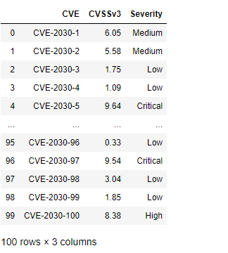
Suppose you have a large DataFrame of scores and want to quickly add a qualitative severity column. the np.select() method is a fast and flexible approach for handling this transformation in a vectorized manner. We can begin by making up some fictional CVEs as our starting dataset

import numpy as np
import pandas as pd
df = pd.DataFrame({"CVE":["CVE-2030-"+ str(x) for x  in range(1,101)],"CVSSv3":(np.random.rand(100)*10).round(2)})

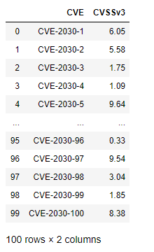
The above is a quick way to build a random DataFrame of made-up CVEs and scores for demonstration purposes. Using np.select() presents a slick vectorized approach to assign them the First.org qualitative label.

Begin by assembling a Python list of conditions based on the First.org labels, and place outcomes in separate Python list.

conditionals = [
    df.CVSSv3 == 0,
    (df.CVSSv3 >0) & (df.CVSSv3 <=3.95),
    (df.CVSSv3 >3.95) & (df.CVSSv3 <=6.95),
    (df.CVSSv3 >= 6.95) & (df.CVSSv3 <=8.95),
    (df.CVSSv3 >= 8.95) & (df.CVSSv3 <= 10)
]

outcomes = ["None","Low","Medium","High","Critical"]

Using the Conditionals

At this point a new qualitative label can be applied to the dataset with one vectorized line of code that invokes the conditionals and labels created above:

df["Severity"] = np.select(conditionals,outcomes)

pd.cut()

An alternative approach, one that is arguably programmatically cleaner but perhaps less flexible, is the Pandas cut() method. There are lot of options for using pd.cut(), so make sure to take some time to review the official documentation to understand the available arguments.

One option is to set up a series of intervals using a Python list. It is important to remember that the intervals will, by default, be closed to the right and open to the left. Below is an initial attempt to pattern intervals after the First.org boundaries

bins = [0,0.01,3.95, 6.95, 8.95, 10]

Now that the boundaries are established, simply add them as arguments in a call to pd.cut()

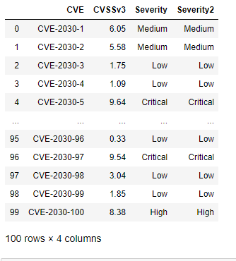
df["Severity2"] = pd.cut(df.CVSSv3,bins, labels=["None","Low","Medium","High","Critical" ], retbins=False)

This results in the following

As always, it is prudent to do some testing: especially to test the boundary conditions. We can redo the array-building exercise while appending a few custom rows at the end using the following code:

np.random.seed(100)
df = pd.DataFrame({"CVE":["CVE-2030-"+ str(x) for x  in range(1,101)],"CVSSv3":(np.random.rand(100)*10).round(2)})
df.loc[len(df.index)] = ['CVE-2030-101', 0] 
df.loc[len(df.index)] = ['CVE-2030-102', 10] 
df.loc[len(df.index)] = ['CVE-2030-103', 0.1] 
df.loc[len(df.index)] = ['CVE-2030-104', 9.0] 
df.loc[len(df.index)] = ['CVE-2030-105', 4.0]
df.loc[len(df.index)] = ['CVE-2030-106', 3.96]
df.tail(10)

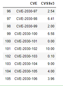
The df.loc[len(df.index)] simply locates the index value needed to add an additional row. Setting a random seed in line 1 above makes the DataFrame reproducible despite the values being randomly generated.

Now, if this were a unit test, then we would assert that CVE-2030-101 would have qualitative value ‘None’ and CVE-2030-106 would have qualitative value ‘Medium’. Note that for readability we can also improve the way we label the columns of the DataFrame to more readily identify the type of binner employed. Running the binner routines results in:

np.random.seed(100)
df = pd.DataFrame({"CVE":["CVE-2030-"+ str(x) for x  in range(1,101)],"CVSSv3":(np.random.rand(100)*10).round(2)})
df.loc[len(df.index)] = ['CVE-2030-101', 0] 
df.loc[len(df.index)] = ['CVE-2030-102', 10] 
df.loc[len(df.index)] = ['CVE-2030-103', 0.1] 
df.loc[len(df.index)] = ['CVE-2030-104', 9.0] 
df.loc[len(df.index)] = ['CVE-2030-105', 4.0]
df.loc[len(df.index)] = ['CVE-2030-106', 3.96]
df["Severity pd.cut()"] = pd.cut(df.CVSSv3,bins, labels=["None","Low","Medium","High","Critical" ])
bins = [0,0.01,3.95, 6.95, 8.95, 10]
df["Severity np.select()"] = np.select(conditionals,outcomes)
df.tail(10)

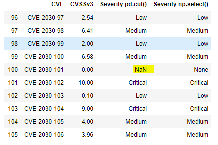
The boundary testing has turned up a problem: the pd.cut() doesn’t handle the value zero because the first interval – 0, 0.1 is open on the left. Such an interval is designated by math types as (0, 0.1], with the parenthesis indicating that zero is not contained in the interval. This bug is easily addressed–the interval can be started at -.99 rather than zero. Alternatively, one could use the method’s arguments to adjust the open-on-left, closed-on-right default behavior.

The pd.cut() bin intervals are adjusted as:

bins = [-.99,0.01,3.95, 6.95, 8.95, 10]

Running the entire code again looks like this:

np.random.seed(100)
df = pd.DataFrame({"CVE":["CVE-2030-"+ str(x) for x  in range(1,101)],"CVSSv3":(np.random.rand(100)*10).round(2)})
df.loc[len(df.index)] = ['CVE-2030-101', 0] 
df.loc[len(df.index)] = ['CVE-2030-102', 10] 
df.loc[len(df.index)] = ['CVE-2030-103', 0.1] 
df.loc[len(df.index)] = ['CVE-2030-104', 9.0] 
df.loc[len(df.index)] = ['CVE-2030-105', 4.0]
df.loc[len(df.index)] = ['CVE-2030-106', 3.96]
bins = [-.99,0.01,3.95, 6.95, 8.95, 10]
df["Severity pd.cut()"] = pd.cut(df.CVSSv3,bins, labels=["None","Low","Medium","High","Critical" ])
df["Severity np.select()"] = np.select(conditionals,outcomes)
df.tail(10)

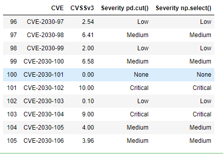
This is the result we were expecting.

Note one other interesting implementation detail; the CVSSv3 mapping from First.org uses precision = 1 and the code and data generation used here was done with precision = 2. That is a detail that may well have led to unexpected results. We could have adjusted the random generator to round to a single digit after the decimal, or simply reset the DataFrame using the round function:

df = df.round(1)

Finishing the NVD JSON MongoDB Mirror

Finishing off the discussion of NVD JSON mirroring: there is a repository available for download here via github including a Jupyter Notebook that contains all of the functionality discussed in the various NVD-CVE blog posts.

To start using the Notebook you must install Mongodb: follow the steps below as a rough roadmap–there are countless platform specific, step-by-step guides available as references on how to install and get started with a Mongodb instance.

  • Install MongoDB
  • Create a database named nvd with two collections: maincol and modscol
  • Create a user than can admin the above db and collections
  • Determine a configuration directory where you will place an environment file for connecting to your mongodb instance
  • Determine a working directory for downloading the NVD files
  • Place a file named “.mongo.env” in the configuration directory of choice (e.g. your home directory). The structure of this file is described in the Jupyter Notebook

To begin, the code contains a method (see below) to download and insert the NVD JSON yearly files into the maincol collection. Next there are routines to update this main collection of CVEs with the modification file that NVD provides. NVD suggests initially downloading the yearly files, then updating them by periodically applying the modifications file–the modifications file will contain both revised and new CVEs. A reasonable automated schedule might be to re-download and reload the nvdcve-1.1-modified.json.zip file once or twice per day. The modifications file goes back eight days–If not reapplied at least every eight days it will fall too far behind. If that happens, the yearly files will need to be re-downloaded and reloaded.

The example images below depict an invocation of the method to load/reload the yearly files from NVD onto your local mirror, and then a method to reload the modification file. In the code below, um is an instance of the UpdateMongo Class defined in the Notebook.

Invoking a method on the Jupyter Notebook to redownload and reload the NVD yearly JSON files
Redownload and reload the modification file

Apply the Modifications File

In order to keep the main collection of CVEs updated, the modifications file must be frequently updated and applied to the main collection. The modifications file, recall, has both new and modified CVEs in it. Applying it essentially means avoiding duplicates by updating CVEs that exist in the main collection, and adding brand new CVEs that exist in the mods file but not in the main collection. The Class method:

<em><span style="color:#389ec0" class="has-inline-color">update_main_from_mods_dataframe()</span></em>

does this. It has ‘dataframe’ at the end of its name to designate that it uses Pandas DataFrames to determine what is common in each collection–versus pymongo routines. I tend to rely on Pandas for anything that looks like ETL (Extract, Transform, Load).

Demonstration of applying the mods file

Download the github repository containing the code, install Mongodb, and follow along in the Notebook to insert and manipulate your CVE mirror. If you can get through the various steps to the point of adding customization for your own environment, you will have become at least somewhat proficient in using Mongodb, Python and Pandas.

What’s Next?

CVE repositories are most useful when you can add environmental components to the scoring as well as Threat Intelligence. The next exploration demonstrates adding more information and local context through a TI and Asset Discovery layer.

Viewing the NVD’s JSON CVE Datafeed as a Pandas Dataframe

The National Vulnerability Database publishes complete CVE (Common Vulnerabilities and Exposures) information as a JSON-formatted data-feed that can be downloaded into a local repository such as MongoDB and/or processed via scripting. Here is a demonstration of how to easily manipulate, format and query this JSON with Python. Begin by downloading the JSON data feed file from the NVD site here.

You will note that the file is deeply nested and challenging to work with without a bit of manipulation. Creating a Pandas Dataframe is perfect for this. I suggest using a Jupyter Notebook to explore the data structure and understand how the nesting might need to be flattened or otherwise organized for your purposes. The Pandas and JSON modules will be very useful.

From a Python perspective, the JSON nesting consists of nested dictionaries. If you simply ‘cat’ or ‘more’ the data file on a command line it will look a bit tangled, but the JSON module helps import it in such a way as to facilitate flattening.

import json
import pandas as pd
# this is the downloaded JSON file from NVD 
# from a Python perspective, it's a list of 
# nested dictionaries and challenging to 
# make sense of  without some manipulation of the nesting
your_path = 'd://projects/scratch/'
nvd_file = 'nvdcve-1.1-modified.json'
with open(your_path + nvd_file) as json_file:
    data = json.load(json_file)

# get rid of the first few lines of 
# meta information and create a list 
# of dictionaries keyed by cve information
cves = data['CVE_Items']
cves[0]
we still see nested dictionaries at this point, but the data is becoming readable
# notice the actual CVE # is buried 
# in nested dictionary as CVE_data_meta:ID
print(cves[0]['cve']['CVE_data_meta']['ID'])


CVE-1999-0143
# extract all the numbers to build 
# as a column in a dataframe
# simplest is to use a list comprehension for this
cve_number_list = [ sub['cve']['CVE_data_meta']['ID'] for sub in cves ] 
df = pd.DataFrame(cves,index=cve_number_list)
# we would like a column that is CVE numbers rather than an index
df = df.rename_axis('cve_number').reset_index()
df
a nicely formatted dataframe, though there is still nested data buried inside

Now we have a nicely formatted Dataframe that allows for searching: here is an example of searching for CVE-2020-7980:

df.loc[df['cve_number'] == 'CVE-2020-7980']
it is simple to query for CVE numbers

Next time we will look at scoring via the vector that is nested in the ‘impact’ column as well as demonstrate how to do look ups on descriptions and scores.

Python, Splunk and Endpoint data (2nd in a Series)

Jupyter

Before delving back into the resulting data from article #1, let’s digress a bit to discuss another great tool for any Python-minded security person–especially for anyone interested in data analysis. Skip this entire section if you are already a Jupyter user. The Jupyter Project is an open-source effort responsible for developing the Jupyter Notebook: a free tool used for code-sharing and visualization sharing that also happens to be a boon to interactive exploration of data and code.

Jupyter supports Python, R and Scala: the languages of choice for people working on Big Data. It’s especially nice for interactive visualization: it takes the place of Ipython for quick and dirty interactive computing. For people who are already set in a good IDE such as Spyder, it might not be as attractive. However, if like me you tend to use VI then Jupyter is a natural tool for interactivity and visualization. Let’s load the Ted Talks dataset from Kaggle into Jupyter as a preliminary exercise.

Plot of distribution of comments associated with Ted talks – data from Kaggle

The ability to interactively create a shareable, presentation -ready graphical plot with this brief snippet of coding gives you some insight into the popularity of Jupyter.

Using Pandas

Pandas is a Python module that provides a tabular data structure called a dataframe. The use of dataframes allows for efficient manipulation of large data sets in a familiar spreadsheet-like row- column orientation. There is a fair amount of nuance and peculiar syntax involved in acquiring mastery of pandas and dataframes, not to mention closely related topics such as visualization and statistical analysis However, simple skills such as dataframe creation, data export and data access are quickly acquired.

Here we look at the size and column headers of the Ted Talks dataframe from above.

If you want a quality in-depth pandas review, Kevin Markham has some fantastic free courses on pandas available on YouTube through his DataSchool. Check out a beginning session and you will be navigating pandas in no time. Also, Wes McKinney–the main author of pandas–has an excellent O’Reilly book on the subject: Python for Data Analysis.

Sysmon Data

Turning back to where we left off with getting Sysmon data from Splunk, we had a resultsReader object from the Splunk SDK and printed out the raw data. We had simply printed out raw results, but instead let’s now create a Pandas dataframe from it. Putting all of the code into Jupyter including the class files we can modify the driver to below.

def main():
    # create a connection to Splunk
    sc = SplunkConnection()
    # run a search
    ss = SplunkSearch(sc.service)
    # define the search in SPL
    query = 'search source="WinEventLog:Microsoft-Windows-Sysmon/Operational"'
    # limit to 10 results (just for demo speed) and set the search
    ss.set_blocking_search(query,10)
    # set to a dataframe
    d = []
    for result in ss.get_search_results():
        d.append(result)
    df = pd.DataFrame(d)
  

Now we have a dataframe that we can explore interactively.

The pandas table as show in Jupyter

A few things become immediately obvious: Splunk Web doesn’t require an explicit ‘search’ command word nor does it display most internal fields, i.e. fields that begin with ‘_’ . It will be necessary to inhibit these by adding a command | fields – _* to the search. It will also be necessary to specify fields that you want to capture to bypass any optimization or ‘fast mode’ behavior that is happening behind the scenes when searching with the SDK. Let’s craft a better search command to simply capture hashes.

search index=sysmon source="WinEventLog:Microsoft-Windows-Sysmon/Operational" | fields Hashes | fields - _* | head 10

This results in:

Jupyter has provided an extra layer of readability to the dataframes making them easy to work with and view. Beyond that, we have a simple way to experiment with searches and interactively craft new ever more useful searches with customized fields and filters for any requirement. The next logical step is to build in some automation while combining the dataframe with threat intelligence information.

If the objective is to send bulk hashes into a service such as VirusTotal, then it would be nice to separate them out into their own columns: a SHA256 column and an MD5 column. With pandas, this is simple.

Creating a new column and populating it with a substring from another column

In this example creating a new column to the dataframe df simply consisted of declaring it with df[‘SHA256’] and populating it with a series of splits inside the Hashes columns to obtain the appropriate substring. The same can be done for the MD5 hash.

Creating a column and populating MD5 hash

The Sysmon config filter file can be applied and reapplied to get any or all hash formats: sysmon -c -h * will provide all hashes including the IMPHASH, which might be useful to find processes that hackers have tried to obfuscate by simple means to avoid AV detection. In the next article we will work with automating submission to VirusTotal using the VirusTotal API.

About Ray Zupancic