Autonomous Systems (ASs) encapsulate an organization’s routing policies on the Internet. They make for interesting study as a candidate for Network Science-style graphing. One reason an AS graph might be worth studying is as a case analysis demonstrating how to quantify failure and attack risk for a connected set of network devices . Many of the ideas can be extended to an interior routing topology within an organization. It is a bit of work to assemble the AS edges into a graph, but fortunately a few people have done this for us and put the results on the Internet. Unfortunately the latest complete version I found is a few years out of date, but the concepts remain the same.
There are plenty of pages dedicated to BGP hacks and security on the web. Check out this recent article on Network World, or this historical article from the Internet Protocol Journal if you want to learn more about securing BGP and the issues involved. The routing infrastructure of a Tier-1 backbone organization is not going to be brought down by a few router hardware failures, though cascading failure is always a concern (e.g. one failure overloads another router…). However, the outcome of a BGP hack is murkier.
Hardware failure is much more likely to bring down a smaller organization using BGP-I have worked at organizations over the years that had only one external facing router (albeit a fault-tolerant one with dual hardware). Likewise smaller shops are more prone to an attack being successful as well–though they are less likely to be targeted. Such a scenarios is not apt to affect other ASs: small organizations are not likely to be transit network that anyone else uses. If they are, they might not know it or want to be.
Finding a Dataset
An example AS dataset assembled into a GML graph is available from Mark Newman’s website. He has a good variety of datasets for study: in this case the data was collected from the Route Views project at the University of Oregon.
If you have trouble loading the graph, It may be necessary to edit out gratuitous spaces in this GML. The following line of networkx will work if you edit out white space (hint, use VIM or other UNIX tools to automate it as there are approx. 285k lines).
- as_graph = nx.read_gml(‘as-22july06.gml’)
Looking at the dataset with networkx we see it has the following characteristics
- Number of nodes: 22963
- Number of edges: 48436
- Average degree: 4.2186
Let’s look at random fluctuations of the size of the major component as a result of taking out incremental slices of nodes (ASs). As you might expect with an Internet AS graph, the major component has the name number of nodes as the whole graph. We can define the increments as follows:
- fractions = np.array(arange(0,1,.02))
This is simply 30 gradations of 0. , 0.02, 0.04, 0.06, 0.08, 0.1 , 0.12, 0.14, 0.16 , … 1. We will degrade the AS nodes by this fraction per iteration and then re-calculate the size of the major component. Then we will graph the iterations and watch the breakdown in connectivity.
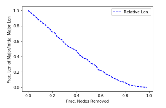
This is a very stable rate of degradation: this indicates the AS network is robust with respect to random failures. Now let’s take a look at what happens in a targeted attack: that is when an attacker chooses what to remove. In most cases a smart attacker will go after hubs, so we can simulate an attack by going after the nodes of highest degree. Using the same fractional increments, we get the follow result for the size of the major component.
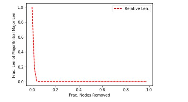
This is a much less stable depiction of failure as nodes are removed. The problem is likely that the AS graph has so-called ‘super-hubs’ that control a lot of connectivity. This can be easily confirmed by looking at a degree distribution and looking at the top ten nodes. Below is the degree distribution. The second figure down is the entire degree distribution using a logarithmic scale.
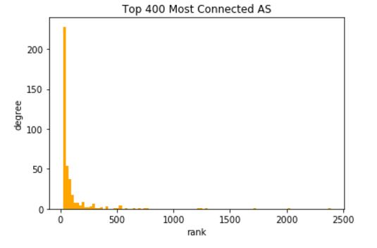
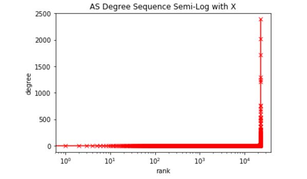
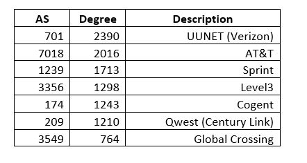
It is easy to see that a few of the 22,000 nodes control a massive amount of connectivity, and the degree distribution is highly stratified into super-hubs. Working out the first few nodes we get the following (remember this is old data):
In Network Science there is a very interesting measure called Betweenness Centrality that alerts to the existence of nodes that do not necessarily have have high degree but are very central in terms of what they connect. On a network, this could be a case where a router with out many connections happens to be very central in connecting two regions. In the case of ASs it comes to mind that smaller degree NAPs (technically now called Internet Exchange Points) or the former Metropolitan Area Ethernets (e.g. MAE-West), or some similar structure might have low degree but high centrality.
For any medium size complex network (e.g. 10,000 to 100,000 nodes) this will be calculation best performed on an engineering workstation as it takes O(n*m) time where n is vertices and m is edges. For much larger networks one would want to consider approximation methods. Here are the results for ASs: 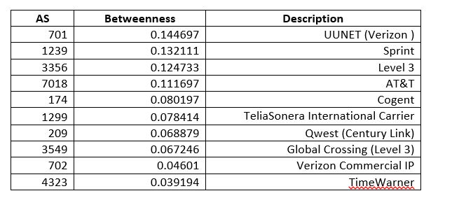
This is interesting for its lack of results–no hidden connector of low degree was found in the top ten. This technique could be valuable for examining connecting devices in an Enterprise, however.
What then is the end result of trying to analyze old AS data? The various measures determined here: rate or random failure, rate of attack-based failure, centrality, and degree are quantifiers in a risk analysis. This removes the guesswork to some degree and informs risk teams of exactly what a device represents. You can Find the Jupyter Notebook code behind these explorations on github here.