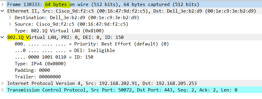
Understanding network traffic flows is a multifaceted subject involving potentially many different tools and utilities. Examining raw capture data in terms of PCAP files can be facilitated with the help of a few common and freely available tools. Data Analysis platforms such as R and Pandas can be helpful as well Packet Capture files are usually viewed and manipulated with the Wireshark GUI, but one can also use tshark–the command line utility that is part of Wireshark. An advantage of tshark lies in its quick ability to glean out statistics and save the data to csv files.
Tip
When capturing data in bulk to profile conversations you may not care if you lose a small percentage of packets. If the goal is to troubleshoot and trace out individual conversations keep in mind the loss rate that might be involved and consider filters: if there is a need to capture much more than a fraction of a 1GbE or 10GbE, then a hardware capture tool may be necessary to avoid significant capture loss. Remember that in the Wireshark family that the dumpcap utility used alone is the least lossy and least resource intensive tool to capture with.
Profiling Frame Lengths
Here is an example set of commands used to derive data from a PCAP using tshark–in this case the frame length.
tshark -nr maccdc2012_00000.pcap -T fields -e frame.len > length_counts.txt
In this case we use a PCAP file (maccdc2012) that is publicly available on the web- this one was created from a hacking competition. The above tshark command populates the file length_counts.txt with the length of each Ethernet frame. This will result in a very large and unwieldy file:
wc -l length_counts.txt
8635943 length_counts.txt
We would like to load the data into a data analysis tool such as R. It should be apparent that there aren’t 8 million possible lengths of an Ethernet frame and therefore the data can be summarized.
Suppose we want to summarize the data for efficiency, and then load it on-demand as a frequency table rather than a line-by-line frame count file. That is, a simple table that depicts the frequency of a given packet length–since there is only going to be around 1500 different lengths based on the definition of Ethernet. That means we would not have all that many lines to contend with. Fortunately in Linux it’s easy to create a frequency table.
more length_counts.txt | sort -n | uniq -c > table_lengths.csv
Here we simply piped the data into a sort in order to place identical data on adjacent lines, and then counted the instances of a given value. Now comes the more challenging task: if we want to analyize or manipulate the data in R-Studio we will need to learn some R commands including the use of a few extra packages not part of the standard default install. Start by adding in the headers of Frequency and Length to the file. Also note that tshark accepts a ‘-E separator=,’ argument to easily output in CSV format.
Frequency,Length
2285, 60
4598604, 64
23, 65
1158960, 66
112, 67
37907, 68
76, 69
…
The following R code can be used once the vcdExtra package is added to your R-Studio:
> FrequencyTable <- read.csv(“table_lengths.csv”, header = TRUE)
> # install the vcdExtra package to get access to the
> # expand.dft function
> dataLengths <- expand.dft(FrequencyTable, freq=”Frequency”)
The above commands have loaded a small frequency table and expanded it into a very large dataset. The data can now be summarized with the summary command–first we ‘coerce’ it into numeric format for ease of manipulation with the as.numeric command.
> mylengthdata <- as.numeric(unlist(dataLengths)
> summary(mylengthdata)
Min. 1st Qu. Median Mean 3rd Qu. Max.
60.0 64.0 64.0 108.3 78.0 1518.0
Tip
The 802.3 and Ethernet specifications have a maximum frame length of 1518 (1522 if VLAN tagging is included), so the above Max. makes sense. When trying to comprehend frame sizes, it is worth noting that hardware can strip off the FCS–hence 1518 might actually include the VLAN tag.
The minimum specification for frame length is 64-bytes. There are a number of reasons why one might see less than 64- bytes: if the frame is very small (e.g. less than 36-bytes) it is likely a runt frame due to an error. Stripping off padding or seeing a frame being sent before padding is applied can also be a culprit. In this case, the 60-byte frames look like normal frames where hardware has stripped the FCS (checksum). The preponderance of 64-byte frames appears to be simply a result of a minimal frame with FCS stripped and 4-byte VLAN tag applied. Taking a look at one reinforces this:
Frame Size Frequency
| Frequency | Size in Bytes |
|---|---|
| 4598604 | 64 |
| 1494722 | 78 |
| 1158960 | 66 |
| 571041 | 70 |
| 101899 | 1438 |
| 47268 | 109 |
| 40986 | 1518 |
| 37907 | 68 |
Plotting a histogram in R with the hist command we can see that, treated as a sample, it’s probability distribution is vaguely similar to the inverse of a Normal distribution with the caveat that the smallest few sizes of frames vastly dominates the other data (53% are 64-byte, etc).
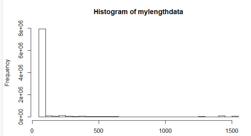
This is an interesting result in that most studies one refers to as far as Internet Mix of packets assumes a bi-modal distribution with very large and very small packets being the spike points. Remember that if traffic is to be characterized in raw volume (bytes versus packets) that a 1500 byte packet is worth 25 minimum-length packets.
Port Analysis
It’s worth noticing the exhaustive options that tshark provides out of the box. A look at the man page for tshark demonstrates some native statistical capability. For example, if a breakdown of web traffic is needed, there is:
![]()
Lets ask tshark for port information so that we can build a frequency table based on ports.
tshark -r maccdc2012_00000 -n -e tcp.srcport -e tcp.dstport -T fields > tcpports2.txt
Now let’s import into Pandas and use Pandas to build a frequency table for low source ports:
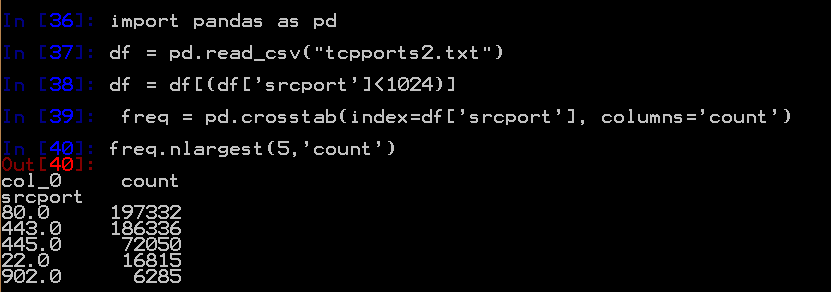
T902 – hmm, maybe ESXi?
Conclusions
Why might this be valuable? Mainly it’s valuable to add a few analysis tools to your toolkit and observe how simple it is to manipulate data back and forth between a utility like tshark and formal data analysis platforms such as R and Pandas. Profiling and understanding network traffic in data-centric ways has countless potential applications.