Excel Archives - Grumblesoft

Many organizations have IP address blocks spread out across the country or world, and must rely on centralized tools that may or may not report location and owner details in as granular a fashion as sometimes required. Splunk can come to the rescue in resolving an IP Address into a location and responsible team. If you work with Splunk you likely have used Lookups to enrich event data,. This is a demonstration of the advanced matching capabilities using CIDR that can save you from trying to deal with networks that don’t end on an octet boundary (e.g. /27s) and thus are harder to deal with in Excel spreadsheets or other tabulation tools.

Excel for sorting IP addresses

As a preliminary, a note on using Excel to manipulate and sort IP addresses. If all of your networks end on an octet boundary, an Excel spreadsheet or Google sheet may be all you need to analyze the IP addresses and locations in your Enterprise . Simply break the full addresses into octets using Text to Columns , sort , and then remove the last column and reassemble. Now if you combine the below steps with a network-to-location lookup table and use the VLOOKUP function, you can quickly create an analysis.

Use Text-to-Columns to create a network cell

However, Excel is not as simple to apply if you use subnets or supernets that don’t fall on an octet boundary. As an alternative approach in your spreadsheet, IP addresses can be converted to either binary or decimal Integers –you can find or wrap your own Visual Basic to resolve them to Integers (e.g. octet1 * 256**3, …) and match them as ranges corresponding to locations. After this conversion it’s simple to sort into corresponding networks.

As an exercise, suppose one wanted to count the number of network-regions in a given output of raw IP addresses. Do the analysis above to sort into networks, then use a COUNTIF function to find the occurrences (as shown in the below formula bar). Use a de-dup to get the final network count. Note that it’s necessary to get the count via the formula, then copy and paste the G column to an adjacent column using values only (otherwise the de-dup will break the count).

Splunk CIDR-based lookup matching

What if your locations don’t neatly break into octet boundaries? Then it’s more work to do this lookup in Excel. Beyond that, it is very useful to stream output with location/owner/… data instantly available for review. Splunk can be used as a more flexible alternative. Here is a scaled down example, suppose your organization has the following IP map:

Suppose also that you have a bulk data set that you have to act on (e.g. break down into locations/owners and create tickets) in the form of a bulk CSV of systems, as below.

You can easily create a Lookup to process the bulk file uploads into any format of report you need. Here is an example of loading the lookup file, subnetmap.csv, and setting the definition.

Lookup definition with advanced options chosen – CIDR match

With the Lookup loaded, simply upload your bulk data file in order to execute searches against it using the enriched events. Here we loaded the file into an index called ip_analysis.

Obviously this only scratches the surface. A bulk data loader is not actually needed: one can apply this to any event data across an Enterprise that can be enriched by location or owner. It would be simple to write a custom app that allows for input lists on the fly to be enriched by location data: a use case might be that one exports a list of non-compliant hosts from a tool such as Tenable Security Center or McAfee ePO and wants to mass-generate tickets.

Of course, any miscellaneous raw Splunk query can be enriched on the fly: it’s also simple to combine the lookup with tags that delineate classes of hardware (e.g. routers). A use case might be to query Splunk for all routers in California, for example.

Linear programming with Excel Solver

Lately, when one hears about modeling data it conjures up visions of Big Data processes where algorithms are constructed to “learn from experience” across expansive datasets with many potential predictive variables. However, most day-to-day business modeling tasks are modest business analyses that rely on traditional Operations Research techniques to inform decision making. For the Security Analyst, it’s not unlikely you will at some point be asked to model (or refer to your organization’s modeling function) some relatively self-contained capacity or risk problem: you may well end up only needing Excel or some simple Python code.

The next few entries deal with bread-and-butter modeling including simple optimization, forecasting and simulation models that anyone can take on even with out statistical training or background. The tools at hand will be Excel Solver Plug-in, Palisade Software’s @Risk Excel Plug-in, and Python’s PuLP library.

Optimization

Business analysts that must make data-driven decisions often rely on the ubiquitous Excel platform for their analysis (for better or worse, end-point computing with Excel drives business). An IT department example might be availability or capacity modeling where one has to optimally distribute a compute load or a series of application across facilities to achieve a specified availability and capacity. Here is an example scenario than spans capacity and cost modeling–it’s easy to see how it might generalize to a number of IT-related contexts.

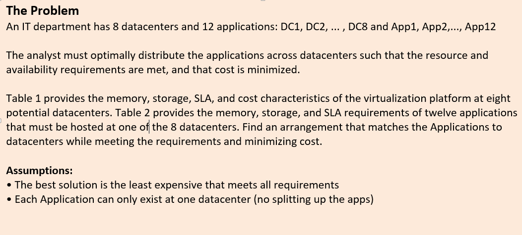
Table 1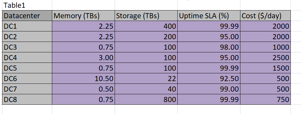

Table 2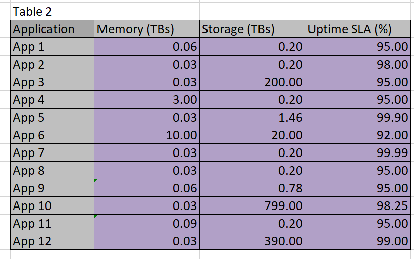

Given the data, we must find a programatic way to solve the optimization problem. The easiest way is with the Excel Solver Add-In. Visit Microsoft’s support site at this link for instructions as to how to find and install the Solver Add-it is freely available and simple to use.

Modeling the problem

There are various techniques for programming this worksheet: one could employ some Visual Basic code, or simply do the calculations with formulas. In this case the task at hand is straightforward enough to rely on simple formulas . We start by defining a grid that maps datacenters to applications using a binary match cell to flag an assignment. This is done in Table 3. Remember, I didn’t put the 1’s and 0’s in–Solver did.

Table 3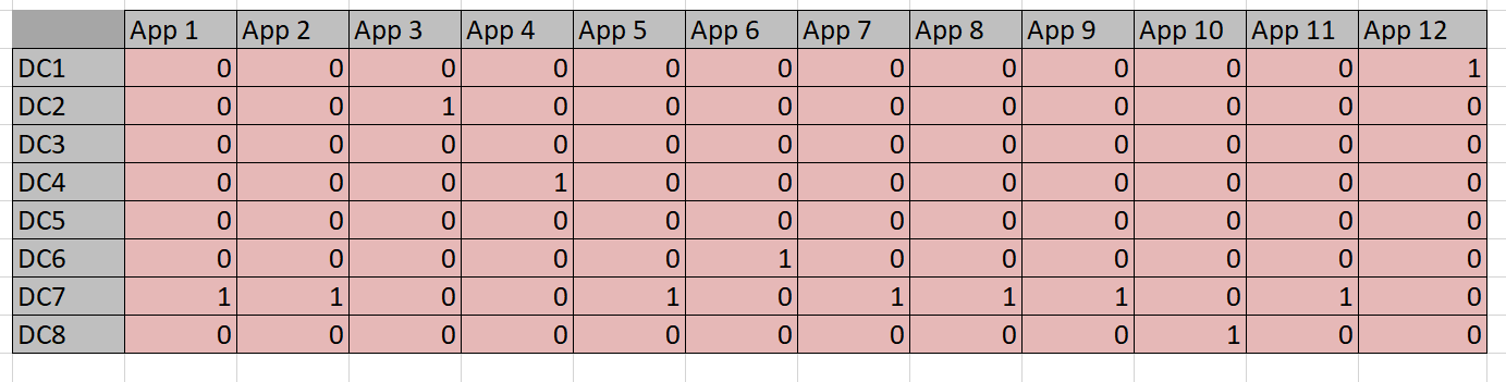

I use light pink in Table 3 to designate cells that are going to be populated by Solver. Above, in Tables 2 and 3, the light purple cells designate the data given to us to work from. The convention here will be to use no color to designate calculated or formula-based cells.

In order for Solver to use the constraints, it must be given access to some calculations on datacenter versus application. For example, the datacenter chosen for App1 must provide for .6 TBs of memory and .2 TBs of storage–if the same datacenter is used for multiple applications, then the sum of the resources needed must not exceed the capability of the datacenter.

This information is added as a constraint to solver as in Diagram 1.

Diagram 1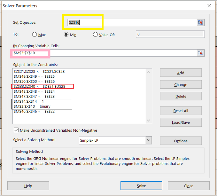

Some examples of what these constraints mean:

red box: storage of apps must sum below the memory capacity of the datacenter
Line 2: storage of the apps must sum below the storage capacity of the datacenter
black box: an app must go to only one datacenter we use a binary table to designate app-to-datacenter assignment (no fractional apps)
the uptime constraints are the 2nd, 3rd, 5th, 6th and 9th lines in the box – a few uptime constraints are left out to reduce the size –it makes no difference to contrain DCs that have uptime of 99.9 as no app can exceed that.

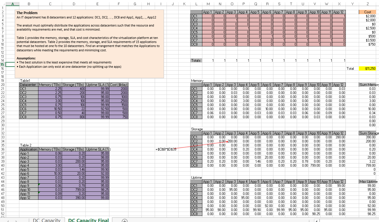
These constraint definitions will make more sense when viewed against the ‘big picture’ in Diagram 4 below: this shows the entire worksheet including row and column names. Below are the constraint calculation tables–the data in these tables is derived via formulas applied to the given data and Solver-chosen data.

Table 4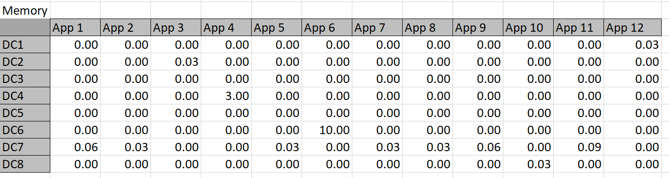

Table 5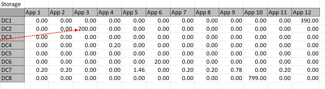

Table 6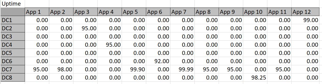

The constraint tables used in this approach are simply copies of Table 3 with the actual memory or storage calculated in cells where Solver chooses to assign an app to a datacenter. For example, Solver might choose to put App 1 in DC 3, so the resources are calculated into the constraint tables. The app columns for DC 3 can then simply be summed up and compared to the actual capacity. Solver works by refining attempts to find the minimal cost solution that meets the resource constraints.

Using the binary constraint serves a couple of purposes: the app doesn’t get broken down fractionally and it also allows for a nice feature of multiplying the assignment (‘1’ if exists, ‘0’ if not) by the resource requirement so we can easily sum up the needed totals. There is also a somewhat more complex reason why it may be desirable to use the seemingly awkward binary structure to model the mappings and constraints-preserving linearity.

Linearity

Excel Solver Plug-In has three algorithms for finding an optimal solution:

Simplex LP
Evolutionary
GRG Nonlinear

The fastest method, and one that guarantees an optimal solution, is Simplex LP (Linear Programming). Our problem as stated can be solved using Linear Programming, which is optimal and fast. If you are wondering about the messy way I constrained the uptime — rather than taking the MAX of a row and doing a simple comparison I took the values in an entire row and compared them to the DC. There is a reason for that: using the MAX function in Excel creates a non-linear constraint.

Those astute at math will note that it’s possible to find a max value of a list using an absolute value (ABS in Excel), but ABS is also non-linear: think about y=|x|, it has to be broken into two cases to be linear. Try to express y=|x| as f(x) = m*x + b, and this will become clear.

Had this model used an ‘If’ statement to decide whether to count memory or storage, that would have also introduced non-linearity; that is the beauty of simply multiplying the value by the binary flag-it allows for a linear representation of the constraint within the calculation.

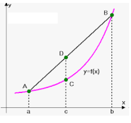
Confused by the desirability of a linear constraint? Think of it this way: convex curves are easy to find optimal solutions on because one will not run into local minima/maxima. If you can present a problem in a linear way, you are guaranteed a fast, optimal solution. If the problem, or the way constraints are modeled, presents non-linearity, then it’s generally a much longer running algorithm and the solution may be only local in nature. Understanding convexity versus non-convexity is a career in itself. Suffice it to say that if one can preserve linearity on simple problems, It’s usually worth the effort to do so even if you must build artifices such as tables built on binary flag multipliers such as was done here.

Diagram 2 – Convexity

The Calculations

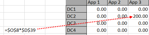
Looking at a formula may make this whole scheme a bit more clear–see Diagram 2. $O$8 will be either ‘1’ or ‘0’ -it represents whether a mapping exists or not. $D$39 is the application storage for App 3.

Diagram 3

Here is the solver result for storage and memory where the yellow cell signifies the objective cell with the total cost minimized. This required only Simplex LP. The solution was arrived at almost instantaneously on a modest desktop computer.

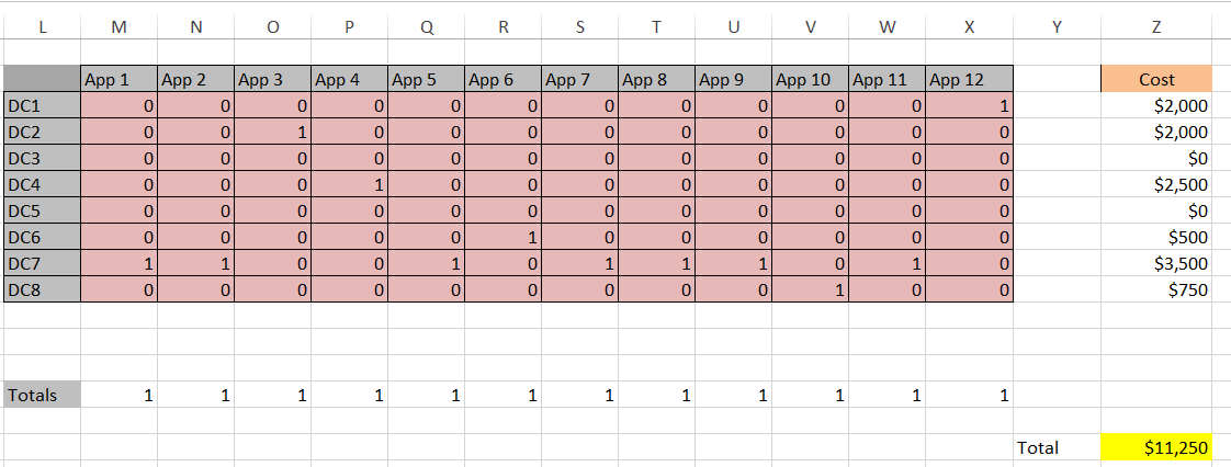
Diagram 4 is the big picture and allows you to see how the constraints actually work in terms of row and column values.

Diagram 4 – the big picture

Here is the link to the file. Needless to say, problems with larger variable sets virtually require a programming tool such as Solver to solve. There are plenty of smaller problems that would be impractical to solve manually as well (this example not so much as I made the values easy to piece into place manually for illustration). Unfortunately, as you get much larger you have to purchase a premium version of Solver or move to another platform.

Grumblesoft

Category Archives: Excel

Splunk Lookups with CIDR Matching